Spiral Matrix II

Problem Definition

LeetCode Link: 59. Spiral Matrix II

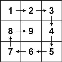
Given a positive integer n, generate an n x n matrix filled with elements from 1 to n² in spiral order.

Example 1:

Input: n = 3
Output: [[1,2,3],[8,9,4],[7,6,5]]

Example 2:

Input: n = 1
Output: [[1]]

Constraints:

1 <= n <= 20

Thought Process

Every time we encounter binary search, it’s always easy to understand but hard to implement, if you want to write a correct binary search, you must adhere to the principle of loop invariants.

Similarly, solving this problem still requires adherence to the principle of loop invariants.

Simulating the process of drawing a matrix in a clockwise direction:

Fill the top row from left to right.
Fill the right column from top to bottom.
Fill the bottom row from right to left.
Fill the left column from bottom to top.

Continue drawing outward in circles.

It can be observed that there are many boundary conditions here. In one iteration, with so many boundary conditions, if we do not traverse according to fixed rules, we will end with a death loop.

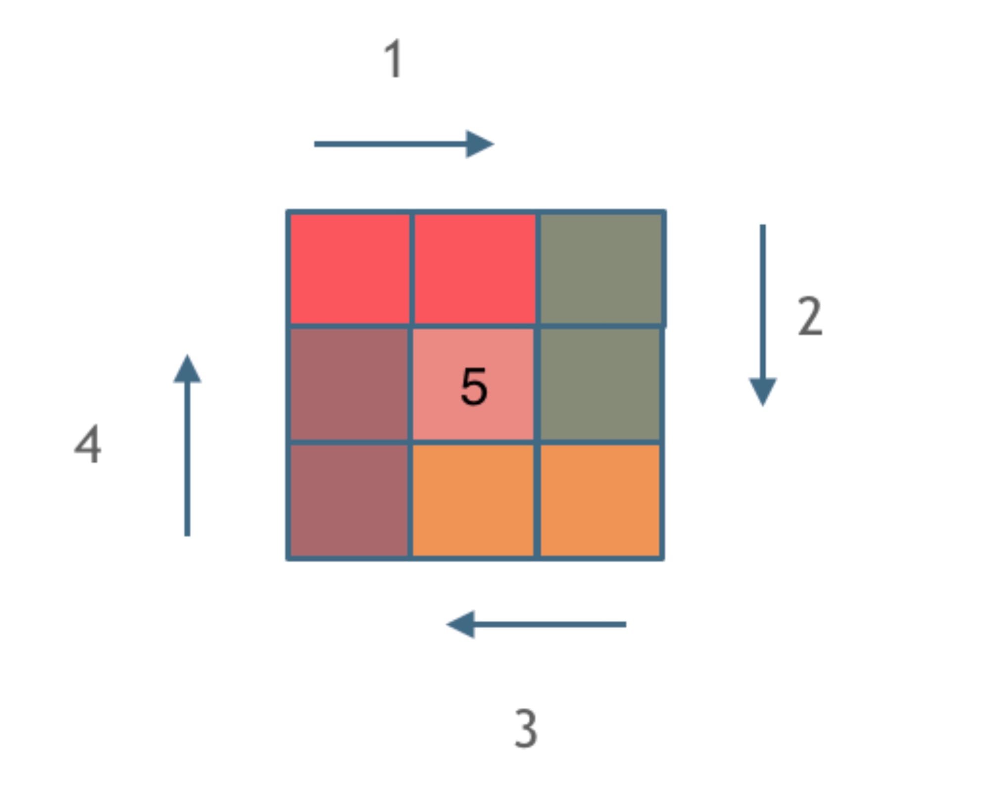
After completing one circle here, we need to draw each of the four edges. How these four edges are drawn is crucial; for each edge drawn, we must consistently follow either a closed-left open-right or open-left closed-right principle so that this entire circle can be drawn according to unified rules.

Now I will draw one circle following the closed-left open-right principle; let’s take a look:

Each color here represents an edge, and the length we traverse allows us to see the handling rules at each corner, where a new edge is given way to continue drawing.

This also adheres to the principle of left-closed and right-open for each edge.

Some people may struggle with this problem because their code becomes increasingly messy as they write it.

This is because when drawing each edge, sometimes it's left-open right-closed, sometimes left-closed right-closed, and then back to left-closed right-open; how can it not get chaotic?

Solution 1

Code

class Solution:
    def generateMatrix(self, n: int) -> List[List[int]]:
        nums = [[0] * n for _ in range(n)]  # Create an n x n matrix filled with zeros
        startx, starty = 0, 0  # Starting point coordinates (top left corner)
        loop, mid = n // 2, n // 2  # Number of loops (layers) to iterate, and the center point if n is odd
        count = 1  # Counter for filling the matrix in order

        # Iterate through each layer, with each layer having an increasing offset
        for offset in range(1, loop + 1):  # Each loop iteration adds an offset, starting from 1
            # Traverse from left to right (top row)
            for i in range(starty, n - offset):  # Left-closed, right-open interval
                nums[startx][i] = count
                count += 1
            # Traverse from top to bottom (right column)
            for i in range(startx, n - offset):  # From top to bottom along the right edge
                nums[i][n - offset] = count
                count += 1
            # Traverse from right to left (bottom row)
            for i in range(n - offset, starty, -1):  # From right to left
                nums[n - offset][i] = count
                count += 1
            # Traverse from bottom to top (left column)
            for i in range(n - offset, startx, -1):  # From bottom to top along the left edge
                nums[i][starty] = count
                count += 1
            # Update the starting point to move inward for the next loop iteration
            startx += 1
            starty += 1

        # If n is odd, fill in the center element of the matrix
        if n % 2 != 0:
            nums[mid][mid] = count
        
        return nums

In the code, loop and mid are both calculated as n // 2 to determine how many layers the matrix has and where the center point is located if n is odd.

Loop (loop = n // 2):
- loop represents the number of concentric layers that need to be filled in the matrix.
- Each layer involves filling numbers from the outer boundaries inward.
- For example, if n = 5, there are 2 complete layers, since 5 // 2 gives 2. These layers are like “onion skins” surrounding the central point.
- Similarly, if n = 4, loop would still be 2 because there are two full concentric layers. The loop variable helps to control how many times you iterate to fully fill the outer boundaries moving inward.
Mid (mid = n // 2):
- mid represents the center point of the matrix when n is odd.
- When n is odd (e.g., n = 5), mid = 5 // 2 = 2. This is the index of the middle element of the matrix (nums[2][2]), which needs to be filled at the end.
- If n is even, there is no single center point, so this mid value is not used directly for a central element.

Thus, both loop and mid are n // 2 to help manage the number of concentric layers (loop) and to identify the center when n is odd (mid). This way, the code can efficiently fill the matrix in a spiral order until all elements are covered, including the center when needed.

offset starts from 1 and goes up to loop + 1 (exclusive), offset essentially represents how far you need to move inward from the boundaries during each iteration of filling the matrix.

Step by step

Let’s go through the steps for n = 5 to see how the matrix is filled step by step.

Initial State:

n = 5
The matrix (nums) is initialized with zeros:

0  0  0  0  0
0  0  0  0  0
0  0  0  0  0
0  0  0  0  0
0  0  0  0  0

loop = n // 2 = 2 (2 complete layers)
mid = 2 (center of the matrix)

Layer 1 (offset = 1):

Top Row (Left to Right)

Starting from startx = 0, starty = 0
Fill from starty to n - offset = 4 (indices 0 to 3)
Fill values: 1, 2, 3, 4
Updated matrix:

1  2  3  4  0
0  0  0  0  0
0  0  0  0  0
0  0  0  0  0
0  0  0  0  0

Right Column (Top to Bottom)

From startx = 0 to n - offset = 4 (indices 0 to 3)
Fill value: 5, 6, 7, 8
Updated matrix:

1  2  3  4  5
0  0  0  0  6
0  0  0  0  7
0  0  0  0  8
0  0  0  0  0

Bottom Row (Right to Left)

From n - offset = 4 to starty = 0 (indices 4 to 1, decrementing)
Fill value: 9, 10, 11, 12
Updated matrix:

1  2  3  4  5
0  0  0  0  6
0  0  0  0  7
0  0  0  0  8
0  12 11 10 9

Left Column (Bottom to Top)

From n - offset = 4 to startx = 0 (indices 4 to 1, decrementing)
Fill value: 13, 14, 15, 16
Updated matrix:

1   2  3  4  5
16  0  0  0  6
15  0  0  0  7
14  0  0  0  8
13  12 11 10 9

Layer 2 follow the similar process

Solution 2

Code

class Solution(object):
    def generateMatrix(self, n):
        if n <= 0:
            return []
        
        # initial the matrix
        matrix = [[0]*n for _ in range(n)]

        # Initialize boundaries and starting value
        top, bottom, left, right = 0, n-1, 0, n-1
        num = 1

        while top <= bottom and left <= right:
            # from left to right
            for i in range(left, right + 1):
                matrix[top][i] = num
                num += 1
            top += 1

            # from top to bottom
            for i in range(top, bottom + 1):
                matrix[i][right] = num
                num += 1
            right -= 1

            # from right to left
            for i in range(right, left - 1, -1):
                matrix[bottom][i] = num
                num += 1
            bottom -= 1

            # from bottom to top
            for i in range(bottom, top - 1, -1):
                matrix[i][left] = num
                num += 1
            left += 1

        return matrix

Key Differences with Solution 1

Layer Management:
- Previous Method: Uses loop and offset to handle each layer. It focuses on progressively reducing the starting points (startx and starty) while calculating the shrinking boundary based on offset.
- Second Method: Uses explicit boundary markers (top, bottom, left, right) and modifies these boundaries after each pass through a direction. This gives a clearer picture of which boundary is being processed at each point.
Approach to Layer Iteration:
- Previous Method: Iterates over each layer by determining an offset, which helps calculate the new boundary for each loop. It also uses startx and starty to manage the inward movement.
- Second Method: Uses while-loop conditions (top <= bottom and left <= right) to control the iteration. This means the layer processing stops when all boundaries overlap, and all cells are filled.
Code Readability:
- Previous Method: Uses multiple for loops with different directions, with calculations involving offset to decide how far the current iteration needs to go.
- Second Method: Uses a series of directional for loops that are easier to visualize and track for each part of the boundary (top, right, bottom, left). This makes it easier to follow the exact path the filling process is taking.
Flow Control:
- Previous Method: Manages each iteration using increasing offsets (offset), which represent how far inward the next layer is located.
- Second Method: Uses dynamic boundary movement (top, bottom, left, right) to directly control how the boundaries shrink as each layer is filled.

Time complexity: O(n^2). Simulating the traversal of a two-dimensional matrix

Space complexity: O(1).

54. Spiral Matrix

Spiral Matrix II

Problem Definition

Thought Process

Solution 1

Code

Step by step

Right Column (Top to Bottom)

Bottom Row (Right to Left)

Left Column (Bottom to Top)

Solution 2

Code

Key Differences with Solution 1

Discussion

Fuel my Writing ⛽

Problem Definition

Thought Process

Solution 1

Code

Step by step

Right Column (Top to Bottom)

Bottom Row (Right to Left)

Left Column (Bottom to Top)

Solution 2

Code

Key Differences with Solution 1

Related Problems

Discussion

Fuel my Writing ⛽