Learning Recommendation Systems: Bayesian Personalized Ranking (BPR)

From rating prediction to personalized ranking: How Bayesian Personalized Ranking (BPR) solves the implicit feedback problem in recommendation systems. A practical guide to better recommendations through pairwise learning.

As a software engineer new to recommendation systems, I initially thought the goal was straightforward: predict a user's rating for an item and simply recommend the ones with the highest scores. However, I quickly learned that this approach has its limitations.
This realization led me to discover Bayesian Personalized Ranking (BPR), a powerful algorithm that reframed my understanding of the recommendation problem from prediction to ranking. In this article, I'll share the key insights I gained from exploring BPR and how it can lead to more effective recommendation systems.The Core Challenge: Personalized Ranking
The Core Challenge: Personalized Ranking
Let me start with the fundamental problem we're trying to solve: personalized ranking. The task is to provide each user with a ranked list of items tailored to their preferences.
Think about it - when you open any recommendation system, you don't just want to know if you'll like something. You want the best items for you ranked at the top, followed by progressively less appealing options. Whether it's:
- Movies ranked by how much you'll enjoy them
- Products sorted by purchase likelihood
- Articles ordered by relevance to your interests
- Songs arranged by how likely you are to listen completely
This ranking aspect is crucial because users typically only engage with the top few recommendations. Getting the order right is everything.
The Problem
When I first started working with recommendation systems, I thought I understood the ranking problem: predict how much someone will like each item, then sort by predicted score. But then I encountered what seemed like a simple dataset and realized something that kept me up at night: most of the data isn't what you think it is.
Consider a typical user interaction dataset:
- User A watched Movie X completely
- User A clicked on Movie Y but stopped after 5 minutes
- User A never interacted with Movie Z
My first instinct was to treat this as a rating prediction problem and then rank by predicted ratings:
- Movie X → Rating: 5 (positive) → Rank high
- Movie Y → Rating: 2 (negative) → Rank low
- Movie Z → Rating: 0 (negative) → Rank very low
But here's the problem: Maybe User A would absolutely love Movie Z - they just haven't discovered it yet! By treating it as negative feedback, I'm teaching my model to rank potentially perfect content at the bottom of their recommendation list.
This is the fundamental challenge of implicit feedback in ranking systems: the absence of interaction doesn't mean negative preference; it might just mean the user hasn't encountered that item yet. But traditional approaches treat missing data as negative signals, completely messing up the ranking order.
The Traditional Approach
My initial approach used pointwise learning - for each user-item pair, predict a score, then rank items by these predicted scores. The model learns by minimizing the difference between predicted and actual ratings.
# Pointwise learning approach:
for user, item in all_pairs:
    predicted_score = model.predict(user, item)
    actual_score = get_rating(user, item)  # 1 if interaction exists, 0 otherwise
    loss += (predicted_score - actual_score)²

# Then rank items by predicted scores
recommendations = sorted(items, key=lambda item: predicted_score[user, item], reverse=True)
The fundamental flaw? When creating rankings, I was treating all unobserved interactions as negative feedback, when in reality they're a mix of:
- True negatives (items the user wouldn't like - should rank low)
- Unknown positives (items the user would love but hasn't seen - should rank high!)
- Items the user is indifferent about (should rank in middle)
By assigning low scores to all unobserved items, I was systematically pushing potentially great recommendations to the bottom of the ranking. This approach optimizes for the wrong objective entirely - it's optimizing rating prediction accuracy, not ranking quality.
Let me show you visually what's happening:
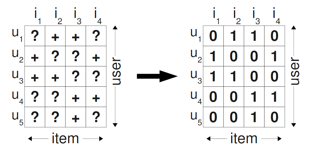
The left side shows our observed data (the interactions we actually see), while the right side shows how traditional approaches fill in the missing data with zeros. The problem is clear: we're treating unknown preferences as negative preferences, which is fundamentally wrong.
Enter BPR
BPR completely reframes the problem. Instead of asking "Will user X like item Y?", it asks:
"Will user X prefer item A over item B?"
This shift from pointwise to pairwise learning is brilliant because:
- Natural for ranking: We care about relative preferences, not absolute scores
- Uses available information: We can confidently say someone prefers items they interacted with over items they ignored
- Avoids false negatives: We don't assume unobserved items are dislikes
Here's what the training data looks like:
# BPR training triplets: (user, preferred_item, less_preferred_item)
training_data = [
    (user_1, item_A, item_B),  # User 1 interacted with A but not B
    (user_1, item_C, item_D),  # User 1 interacted with C but not D
    (user_2, item_A, item_E),  # User 2 interacted with A but not E
    # ... and so on
]
Each triplet represents a preference: we're confident the user prefers the first item over the second.
Here's how this looks visually:
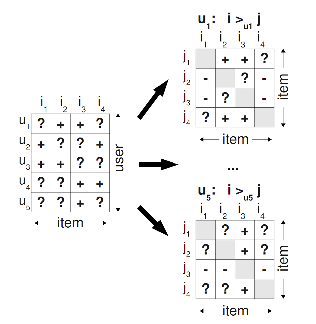
In this pairwise preference matrix:
- + indicates the user prefers the row item over the column item
- - indicates the user prefers the column item over the row item
- ? indicates unknown preferences (what we need to predict)
The key insight is that we only train on the + and - cases where we have confidence about the preference direction. The ? cases are exactly what our trained model will predict during recommendation.
The Mathematical of BPR
Now for the fun part - the math behind BPR is actually quite elegant once you understand the intuition.
Modeling Preference Probability
BPR models the probability that user u prefers item i over item j using the logistic sigmoid:
P(user u prefers item i over item j) = σ(x_ui - x_uj)Where:
x_ui= predicted preference score for user u and item ix_uj= predicted preference score for user u and item jσ(z) = 1/(1 + e^(-z))= sigmoid function
Think of the sigmoid as a "confidence converter". If x_ui - x_uj is:
- Large positive number → High probability (close to 1)
- Near zero → Uncertain (probability ≈ 0.5)
- Large negative number → Low probability (close to 0)
The Objective Function
BPR wants to maximize the likelihood of observing the preference data. For all observed triplets, we want to maximize:
∏ P(user u prefers item i over item j) = ∏ σ(x_ui - x_uj)Taking the log (for numerical stability) and adding regularization:
J = Σ log(σ(x_ui - x_uj)) - λ||θ||²This objective function beautifully captures what we want:
- First term: Maximize probability of correct preferences
- Second term: Regularization to prevent overfitting
Matrix Factorization: Learning Hidden Features
The key insight is how we compute x_ui. BPR uses matrix factorization to represent users and items as vectors in a shared latent space:
x_ui = w_u · h_i (dot product of user and item vectors)Where:
w_u= k-dimensional vector representing user u's preferencesh_i= k-dimensional vector representing item i's characteristicsk= number of latent factors (hyperparameter)
The beauty is that these vectors are learned automatically! The algorithm discovers hidden patterns like:
- User factors: [comedy_preference, action_preference, short_content_preference, ...]
- Item factors: [is_comedy, is_action, content_length, ...]
Stochastic Gradient Descent
To optimize this objective, BPR uses stochastic gradient descent. For each triplet (u, i, j):
- Compute current preference difference:
x_uij = x_ui - x_uj - Calculate prediction error using sigmoid
- Update user and item vectors to reduce error
The update rules are:
w_u ← w_u + α[(1 - σ(x_uij))(h_i - h_j) - λw_u]
h_i ← h_i + α[(1 - σ(x_uij))w_u - λh_i]
h_j ← h_j + α[(1 - σ(x_uij))(-w_u) - λh_j]
Where α is the learning rate and λ is the regularization parameter.
Implementing BPR
Let me walk through my implementation using the Cornac library, which provides an excellent BPR implementation.
Data Preparation
import cornac
import pandas as pd
from recommenders.datasets import movielens
from recommenders.datasets.python_splitters import python_random_split

# Load MovieLens dataset
data = movielens.load_pandas_df(
    size='100k',
    header=["userID", "itemID", "rating"]
)

# Split into train/test
train, test = python_random_split(data, 0.75)

# Create Cornac dataset - this automatically handles triplet generation
train_set = cornac.data.Dataset.from_uir(
    train.itertuples(index=False),
    seed=42
)

print(f'Number of users: {train_set.num_users}')
print(f'Number of items: {train_set.num_items}')
The Dataset.from_uir() method is doing the heavy lifting - it's creating all those (user, preferred_item, less_preferred_item) triplets from our interaction data.
Model Configuration
bpr = cornac.models.BPR(
    k=200,              # Number of latent factors
    max_iter=100,       # Training iterations
    learning_rate=0.01, # Step size for gradient descent
    lambda_reg=0.001,   # Regularization strength
    verbose=True,
    seed=42
)
Let me explain each parameter:
- k=200: Dimensionality of user/item vectors. Higher values can capture more complex patterns but require more computation and risk overfitting.
- max_iter=100: Number of passes through the training data. More iterations generally improve performance but with diminishing returns.
- learning_rate=0.01: Controls how aggressively we update parameters. Too high risks overshooting; too low means slow convergence.
- lambda_reg=0.001: Regularization prevents overfitting by penalizing large parameter values.
Training Process
from recommenders.utils.timer import Timer

with Timer() as t:
    bpr.fit(train_set)
print(f"Training took {t} seconds")
During training, I could see the progress:
100%|██████████| 100/100 [00:01<00:00, 73.33it/s, correct=92.09%, skipped=9.09%]
Optimization finished!
Training took 1.3786 seconds
That "correct=92.19%" means that in 92% of the sampled triplets, our model correctly predicted the user's preference. The "skipped" percentage refers to triplets that were filtered out during sampling.
Making Predictions
from recommenders.models.cornac.cornac_utils import predict_ranking

# Generate rankings for all users
with Timer() as t:
    predictions = predict_ranking(
        bpr, train,
        usercol='userID',
        itemcol='itemID',
        remove_seen=True  # Don't recommend items user has already seen
    )
print(f"Prediction took {t} seconds")
The predict_ranking function generates preference scores for all user-item pairs and returns the top recommendations for each user.
Evaluation Metrics
from recommenders.evaluation.python_evaluation import (
    map, ndcg_at_k, precision_at_k, recall_at_k
)

k = 10
eval_map = map(test, predictions, col_prediction='prediction', k=k)
eval_ndcg = ndcg_at_k(test, predictions, col_prediction='prediction', k=k)
eval_precision = precision_at_k(test, predictions, col_prediction='prediction', k=k)
eval_recall = recall_at_k(test, predictions, col_prediction='prediction', k=k)

print(f"MAP: {eval_map:.3f}")
print(f"NDCG: {eval_ndcg:.3f}")
print(f"Precision@{k}: {eval_precision:.3f}")
print(f"Recall@{k}: {eval_recall:.3f}")
My results:
- MAP: 0.109 - Mean Average Precision across all users
- NDCG: 0.403 - Normalized Discounted Cumulative Gain
- Precision@10: 0.355 - 35.5% of top-10 recommendations were relevant
- Recall@10: 0.180 - Captured 18% of all relevant items in top-10
These metrics might seem modest, but recommendation is inherently difficult - even small improvements can have significant business impact.
What I Learned About BPR's Strengths and Limitations
Strengths
1. Natural for Ranking Problems
BPR directly optimizes for what we care about - relative item ordering rather than absolute scores.
2. Handles Implicit Feedback Well
By using pairwise preferences, BPR avoids the false negative problem that plagues pointwise methods.
3. Computationally Efficient
Matrix factorization scales well, and stochastic gradient descent allows for online learning.
4. Theoretical Foundation
The Bayesian formulation provides a principled approach with clear probabilistic interpretation.
Limitations
1. Cold Start Problem
New users or items have no interaction history, making it hard to generate meaningful recommendations.
2. Popularity Bias
Popular items tend to get recommended more often, potentially creating filter bubbles.
3. Static Preferences
BPR treats all interactions equally regardless of when they occurred, ignoring preference evolution.
4. Limited Context
Basic BPR only uses user-item interactions, ignoring rich contextual information.
Real-World Applications and Extensions
BPR's principles apply broadly across recommendation scenarios:
E-commerce: Amazon uses similar pairwise learning for product recommendations, comparing items users purchased vs. items they viewed but didn't buy.
Streaming Services: Netflix and Spotify leverage these concepts for content ranking, though they've extended far beyond basic BPR.
Social Media: Platforms like TikTok, Instagram, and Facebook use pairwise learning concepts in their feed ranking algorithms, comparing posts users engage with vs. posts they scroll past.
Search Engines: Google's learning-to-rank algorithms employ similar pairwise approaches for search result ordering.
The key insight - that ranking is fundamentally about relative preferences rather than absolute scores - has influenced countless recommendation systems across the industry.
Key Takeaways
After diving deep into BPR, here are the most important lessons I learned:
1. Problem Formulation Matters More Than Algorithm Choice
The shift from pointwise to pairwise learning isn't just a technical detail - it's a fundamental reframing of the recommendation problem.
2. Implicit Feedback Requires Special Treatment
Don't treat missing interactions as negative feedback. The absence of data is not data about absence.
3. Evaluation is Complex
Unlike supervised learning with clear ground truth, recommendation evaluation requires careful thought about what constitutes "success."
4. Simple Ideas Can Be Powerful
BPR's core insight is remarkably simple, yet it had a major impact on recommendation systems. Sometimes the best solutions are elegant rather than complex.
5. Theory Enables Practice
Understanding the mathematical foundation helped me debug issues, tune hyperparameters, and extend the algorithm for specific use cases.
Implementation Tips and Tricks
Through my experiments, I discovered several practical insights:
Hyperparameter Tuning
- Start with
k=50-100for initial experiments learning_rate=0.01works well as a starting point- Increase
lambda_regif you see overfitting - Monitor both training speed and final performance
Data Preprocessing
- Remove users/items with very few interactions
- Consider implicit negative sampling strategies
- Balance your triplet sampling to avoid bias
Computational Considerations
- Use sparse matrix representations for large datasets
- Consider mini-batch SGD for better parallelization
- Implement early stopping based on validation performance
Conclusion
Learning BPR fundamentally changed how I approach recommendation problems. It taught me that the key to good recommendations isn't just better algorithms - it's asking the right questions about the ranking task.
The shift from "How much will this user like this item?" to "Which item will this user prefer?" seems subtle, but it's actually quite significant. It's the difference between trying to predict absolute preferences (nearly impossible with implicit data) and learning relative preferences (much more tractable and directly relevant to ranking).
BPR also showed me the power of mathematical elegance. The core algorithm is conceptually simple, yet it provides a principled foundation that has influenced countless recommendation systems. From e-commerce giants to social media platforms, the insights from BPR continue to shape how we think about ranking and recommendation.
Most importantly, BPR taught me to think carefully about the problem I'm trying to solve before diving into implementation. In this case, recognizing that personalized ranking is fundamentally about relative preferences, not absolute ratings, led to a much better approach. The right problem formulation is often more valuable than the most sophisticated algorithm.
As I continue exploring more advanced techniques like neural collaborative filtering and deep reinforcement learning for recommendations, I keep coming back to the fundamental insights I learned from BPR. It's a testament to the algorithm's enduring value - not just as a practical tool, but as a way of thinking about the recommendation problem.
Discussion