Learning Recommendation Systems: Bilateral Variational Autoencoder (BiVAE)

Discover BiVAE: the breakthrough recommendation algorithm that handles user-item interactions symmetrically, solving key limitations in traditional VAE approaches for better collaborative filtering results.

As I've been working through different recommendation algorithms, I recently studied Bilateral Variational Autoencoders (BiVAE), which was presented at WSDM'21. It's a natural extension of traditional VAE approaches that addresses some fundamental limitations in how we handle user-item interaction data.
If you're learning recommendation systems, BiVAE is worth understanding because it demonstrates how to properly handle the two-sided nature of collaborative filtering data. Let me walk through the algorithm in detail, covering both the theory and implementation.
Understanding Dyadic Data and Its Challenges
Recommendation systems work with what's called dyadic data - data involving measurements between pairs of elements from two distinct sets. In our case, these are users and items, with interactions like ratings, clicks, or purchases.
Here's a simple example of dyadic data:
Interaction matrix R^(U×I):
        Movie1  Movie2  Movie3  Movie4  ...
User1     5      ?       3       1     ...
User2     ?      4       ?       5     ...
User3     2      1       5       ?     ...
User4     4      ?       2       3     ...
...      ...    ...     ...     ...    ...
The key insight is that there are naturally two ways to view this data:
- By users (row-wise): What does User1's rating pattern tell us about their preferences?
- By items (column-wise): What does Movie1's rating pattern tell us about its characteristics?
Both perspectives contain valuable information. A user's rating vector r_u* reveals their preferences, while an item's rating vector r_*i reveals how different user segments respond to that item.
The Matrix Factorization Foundation
Traditional collaborative filtering approaches like matrix factorization handle this naturally by learning latent factors for both users and items:
R ≈ U × V^TWhere U contains user factors and V contains item factors. This symmetric treatment works well and has been the foundation of many successful systems.
The Problem with Neural Approaches
When we moved to neural networks, particularly Variational Autoencoders (VAE), we lost this symmetry. Standard VAE approaches treat the problem asymmetrically:
User-VAE approach:
- Users get explicit latent representations learned by neural encoders
- Items are treated as features in the user's input vector
- Only captures user-side uncertainty and patterns
Item-VAE approach:
- Items get explicit latent representations learned by neural encoders
- Users are treated as features in the item's input vector
- Only captures item-side uncertainty and patterns
This asymmetry is problematic because:
- Information loss: We're not fully utilizing the two-way nature of the data
- Limited extensibility: Hard to incorporate auxiliary information symmetrically
- Modeling mismatch: The model doesn't reflect the true bilateral nature of interactions
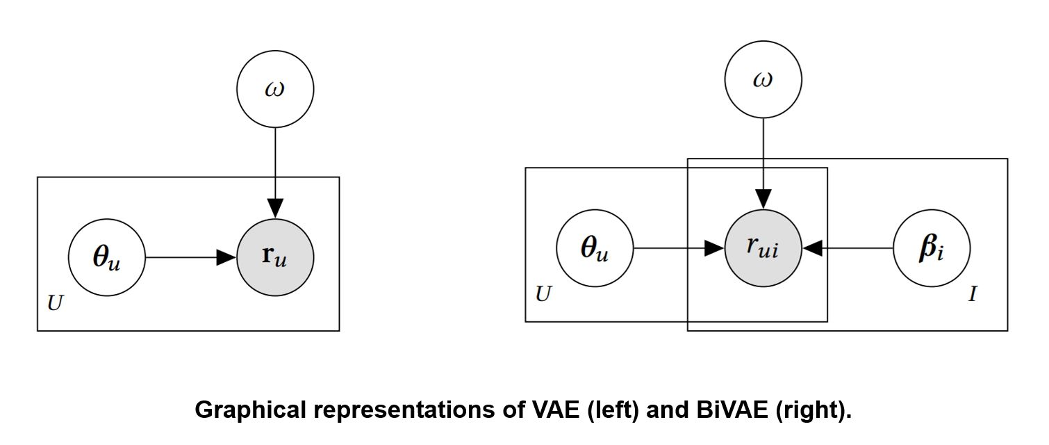
BiVAE: Restoring the Bilateral Nature
BiVAE addresses these issues by treating users and items symmetrically, giving both sides explicit latent representations learned through coordinated neural networks.
Mathematical Formulation
Let me walk through the mathematical foundation step by step.
Notation and Setup
- R: User-item interaction matrix of size U×I
- r_ui: Interaction between user u and item i (rating, click, etc.)
- r_u*: Row vector representing all interactions for user u
- *r_i: Column vector representing all interactions for item i
- θ_u ∈ R^K: Latent representation for user u
- β_i ∈ R^K: Latent representation for item i
- K: Dimensionality of latent space
How BiVAE Works: From Intuition to Mathematics
Let me explain BiVAE starting with the big picture, then diving into the necessary math.
The Big Picture
Imagine you're trying to understand why people like certain movies. BiVAE's key insight is that we need to model both sides of the interaction:
- Users have hidden preferences - like [Action: high, Romance: low, Comedy: medium]
- Movies have hidden characteristics - like [Action: high, Romance: low, Comedy: low]
- Ratings happen when preferences meet characteristics
The "bilateral" part means we give both users AND movies their own neural networks to learn these hidden patterns, instead of only focusing on one side like traditional VAE.
The Mathematical Foundation
Now let's see how this translates to math. Don't worry - I'll connect each formula back to the intuition.
Step 1: Defining Our Hidden Representations
Each user u gets a hidden preference vector θ_u, and each item i gets a hidden characteristic vector β_i. Both are K-dimensional (where K might be 50, representing 50 different "factors" like action, romance, etc.).
Step 2: The Generative Story (How Ratings Are Born)
BiVAE tells a probabilistic story about how a rating r_ui between user u and item i comes to exist:
Prior distributions (starting assumptions):
p(θ_u) = N(0, I)  # User preferences start from a neutral baseline
p(β_i) = N(0, I)  # Item characteristics start from a neutral baseline
What this means: Before seeing any data, we assume users and items start with "average" characteristics. This prevents overfitting and helps with new users/items.
Interaction generation:
p(r_ui|θ_u, β_i) = EXPFAM(r_ui; η(θ_u, β_i, ω))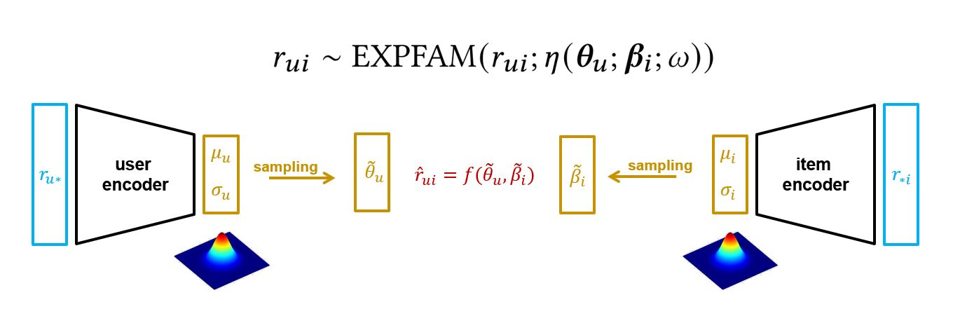
What this means: Given a user's preferences θ_u and an item's characteristics β_i, the rating r_ui is generated from some probability distribution. The function η combines the user and item vectors - it could be as simple as their dot product (θ_u^T β_i) or a more complex neural network.
The "exponential family" part is flexible and includes:
- Poisson: For count data (views, clicks)
- Gaussian: For star ratings (1-5 stars)
- Bernoulli: For like/dislike data
Step 3: The Learning Challenge (Working Backwards)
In reality, we see the ratings and want to figure out the hidden user preferences and item characteristics. This is where things get tricky mathematically.
We want to compute: p(θ_{1:U}, β_{1:I}|R) - "What are the user preferences and item characteristics, given all the ratings we observed?"
The problem: This is mathematically intractable (impossible to compute exactly) because users and items are all interconnected.
BiVAE's solution: Use variational inference - approximate the true answer with something we can compute.
The Inference Model (The Neural Network Part)
Instead of computing the exact answer, BiVAE learns to approximate it using neural networks:
# User encoder: looks at a user's ratings and guesses their preferences
q(θ_u|r_u*) = N(μ_ψ(r_u*), σ_ψ(r_u*))

# Item encoder: looks at an item's ratings and guesses its characteristics
q(β_i|r_*i) = N(μ_φ(r_*i), σ_φ(r_*i))
What this means:
- μ_ψ and σ_ψ are neural networks that take a user's rating vector as input
- They output the mean and standard deviation of a Gaussian distribution
- This distribution represents our "best guess" about the user's hidden preferences
- Same logic applies to items with μ_φ and σ_φ
Key insight: Instead of a single point estimate ("User1 likes action exactly 0.8"), we get a distribution ("User1 likes action around 0.8, give or take 0.2"). This uncertainty is crucial for handling sparse data.
The Training Objective: ELBO
BiVAE optimizes something called the Evidence Lower BOund (ELBO):
L = Σ_{u,i} E_q[log p(r_ui|θ_u, β_i)]           # Reconstruction term
    - Σ_u KL(q(θ_u|r_u*)||p(θ_u))               # User regularization
    - Σ_i KL(q(β_i|r_*i)||p(β_i))               # Item regularization
Breaking this down:
- Reconstruction term: "How well can we predict the actual ratings using our learned user preferences and item characteristics?"
- User regularization: "Don't let user preferences get too extreme - keep them reasonably close to the neutral starting point"
- Item regularization: "Don't let item characteristics get too extreme either"
This balances accuracy (fitting the data) with generalization (not overfitting).
The Reparameterization Trick
To train neural networks, we need gradients to flow through the sampling process. The reparameterization trick makes this possible:
# Instead of directly sampling from the distribution
θ_u ~ N(μ_ψ(r_u*), σ_ψ(r_u*))

# We rewrite it as:
ε ~ N(0, I)  # Sample from standard normal
θ̃_u = μ_ψ(r_u*) + σ_ψ(r_u*) ⊙ ε  # Transform to get our sample
What this achieves: Now gradients can flow through μ_ψ and σ_ψ during backpropagation, enabling us to train the neural networks.
Alternating Optimization: The Training Strategy
Here's where BiVAE gets clever. Instead of trying to optimize everything at once, it alternates:
For each epoch:
    # Phase 1: Fix item parameters φ, optimize user parameters ψ
    For each user batch:
        # Sample user representations using current user encoder
        θ̃_u = μ_ψ(r_u*) + σ_ψ(r_u*) ⊙ ε

        # Calculate loss focusing on user-related terms
        loss = reconstruction_loss + user_KL_penalty

        # Update user encoder parameters ψ
        update_user_encoder(loss)

    # Phase 2: Fix user parameters ψ, optimize item parameters φ
    For each item batch:
        # Sample item representations using current item encoder
        β̃_i = μ_φ(r_*i) + σ_φ(r_*i) ⊙ ε

        # Calculate loss focusing on item-related terms
        loss = reconstruction_loss + item_KL_penalty

        # Update item encoder parameters φ
        update_item_encoder(loss)
Why alternating works better:
- Computational efficiency: Easier to optimize smaller subproblems
- Memory management: Don't need to store gradients for all parameters simultaneously
- Training stability: Less chaotic than joint optimization
- Practical scalability: Can handle larger datasets more easily
Connecting Math Back to Intuition
Let's connect these mathematical concepts back to our movie example:
- θ_u = [0.8, -0.2, 0.5]: User1 loves action (0.8), dislikes romance (-0.2), neutral on comedy (0.5)
- β_i = [0.9, 0.1, 0.2]: Movie1 is heavy action (0.9), light romance (0.1), light comedy (0.2)
- η(θ_u, β_i) = θ_u^T β_i = 0.8×0.9 + (-0.2)×0.1 + 0.5×0.2 = 0.8: High score suggests User1 will like Movie1
- Neural encoders: Instead of guessing these numbers randomly, the neural networks learn to predict them by looking at rating patterns
- Uncertainty: Instead of θ_u = [0.8, -0.2, 0.5] exactly, we might have θ_u ~ N([0.8, -0.2, 0.5], [0.1, 0.1, 0.1]) - we're confident about the values but acknowledge some uncertainty
The math provides the rigorous foundation, but the intuition helps us understand what's actually happening.
Implementation Deep Dive
Now let's see how this translates to working code:
Data Preparation and Setup
import os
import sys
import torch
import cornac
from recommenders.datasets import movielens
from recommenders.datasets.python_splitters import python_random_split
from recommenders.models.cornac.cornac_utils import predict_ranking
from recommenders.evaluation.python_evaluation import (
    map, ndcg_at_k, precision_at_k, recall_at_k,
)

# Load MovieLens data
data = movielens.load_pandas_df(
    size='100k',  # Can be '100k', '1m', '10m', or '20m'
    header=["userID", "itemID", "rating"]
)

print(f"Dataset shape: {data.shape}")
print(data.head())

# Split data randomly (75% train, 25% test)
train, test = python_random_split(data, 0.75)
Creating the Cornac Dataset
Before we can train BiVAE, we need to convert our pandas DataFrame into a format that Cornac understands. Let's see what we're working with first:
# Let's look at our training data format
print("Training data sample:")
print(train.head())
print(f"Training data shape: {train.shape}")
This shows something like:
Training data sample:
       userID  itemID  rating
98980     811     901     4.0
69824     804     755     3.0
9928       52     287     5.0
75599     735     181     4.0
95621     897      96     5.0
Training data shape: (75000, 3)
Now we convert this to Cornac's internal format:
# Create Cornac dataset object
train_set = cornac.data.Dataset.from_uir(
    train.itertuples(index=False),  # Convert DataFrame rows to tuples
    seed=42                         # For reproducible results
)

print(f'Number of users: {train_set.num_users}')
print(f'Number of items: {train_set.num_items}')
print(f'Number of ratings: {len(train)}')  # Use original DataFrame length

# Alternative: if you want to get it from the dataset object
# print(f'Number of ratings: {train_set.matrix.nnz}')  # nnz = number of non-zeros
What's happening here:
train.itertuples(index=False): Converts each row of our DataFrame into a tuple like (userID, itemID, rating). Theindex=Falsemeans we don't include the row index number.from_uir: Stands for "from User-Item-Rating" - Cornac expects data in this triplet format.seed=42: Sets a random seed so we get consistent results every time we run the code. The number 42 is arbitrary (it's a programming joke), but keeping it consistent helps with debugging.
What Cornac does internally:
- Maps user and item IDs to internal integer indices (0, 1, 2, ...)
- Creates efficient data structures for training
- Handles sparse matrix representations
- Provides useful iterators we'll use during training
The output might look like:
Number of users: 943
Number of items: 1642
Number of ratings: 75000
Model Configuration and Training
# Model hyperparameters
LATENT_DIM = 50          # Dimension of θ_u and β_i
ENCODER_DIMS = [100]     # Hidden layer sizes for encoders
ACT_FUNC = "tanh"        # Activation function
LIKELIHOOD = "pois"      # Exponential family choice (Poisson)
NUM_EPOCHS = 500         # Training epochs
BATCH_SIZE = 128         # Mini-batch size
LEARNING_RATE = 0.001    # Learning rate

# Initialize BiVAE model
bivae = cornac.models.BiVAECF(
    k=LATENT_DIM,                    # Latent dimensionality
    encoder_structure=ENCODER_DIMS,   # Encoder architecture
    act_fn=ACT_FUNC,                 # Activation function
    likelihood=LIKELIHOOD,            # Likelihood function
    n_epochs=NUM_EPOCHS,             # Training epochs
    batch_size=BATCH_SIZE,           # Batch size
    learning_rate=LEARNING_RATE,     # Learning rate
    seed=42,                         # Random seed
    use_gpu=torch.cuda.is_available(), # GPU usage
    verbose=True                     # Print training progress
)

# Train the model
from recommenders.utils.timer import Timer
with Timer() as t:
    bivae.fit(train_set)
print(f"Training took {t} seconds")
Making Predictions and Evaluation
# Generate ranking predictions for all users
with Timer() as t:
    all_predictions = predict_ranking(
        bivae,
        train,
        usercol='userID',
        itemcol='itemID',
        remove_seen=True  # Don't recommend items users have already seen
    )
print(f"Prediction took {t} seconds")

# Evaluate using standard metrics
TOP_K = 10

eval_map = map(test, all_predictions, col_prediction='prediction', k=TOP_K)
eval_ndcg = ndcg_at_k(test, all_predictions, col_prediction='prediction', k=TOP_K)
eval_precision = precision_at_k(test, all_predictions, col_prediction='prediction', k=TOP_K)
eval_recall = recall_at_k(test, all_predictions, col_prediction='prediction', k=TOP_K)

print(f"MAP@{TOP_K}: {eval_map:.6f}")
print(f"NDCG@{TOP_K}: {eval_ndcg:.6f}")
print(f"Precision@{TOP_K}: {eval_precision:.6f}")
print(f"Recall@{TOP_K}: {eval_recall:.6f}")
Understanding the Results
For MovieLens 100k, typical results might look like:
Prediction took 0.9817 seconds
MAP@10: 0.144588
NDCG@10: 0.473117
Precision@10: 0.412739
Recall@10: 0.224707
These metrics tell us:
- MAP: Average precision across all users - higher is better
- NDCG: Ranking quality with position discounting - higher is better
- Precision@10: Fraction of top-10 recommendations that are relevant
- Recall@10: Fraction of relevant items found in top-10
Practical Considerations
Hyperparameter Tuning
Key parameters to experiment with:
Latent Dimensionality (k):
- Smaller values (20-50): Faster training, less overfitting, might underfit
- Larger values (100-200): More expressive, slower training, potential overfitting
Encoder Architecture:
- Single layer: Simple, fast, might be too limited
- Multiple layers: More expressive, slower, requires more tuning
Likelihood Function:
- "pois": Good for count data (views, clicks)
- "bern": Good for binary data (like/dislike)
- "gaus": Good for continuous ratings
Learning Rate and Epochs:
- Start with 0.001, adjust based on convergence
- Monitor training loss to avoid over/underfitting
Computational Requirements
BiVAE is more computationally intensive than traditional methods:
Training Time: Expect significantly longer training than matrix factorization
Memory Usage: Scales with number of users + items + interactions
GPU Benefits: Neural network components benefit greatly from GPU acceleration
When to Use BiVAE
BiVAE is most beneficial when:
- Rich interaction data: Sufficient user-item interactions for neural training
- Auxiliary information: You want to incorporate side information from both users and items
- Sparse data benefits: The probabilistic approach helps with uncertainty
- Non-linear patterns: Linear methods like matrix factorization are insufficient
- Computational resources: You can afford the extra training time
Consider alternatives like matrix factorization or simpler neural approaches if:
- Data is extremely sparse
- Training time is critical
- Interpretability is important
- Dataset is small
Real-World Applications
The bilateral nature of BiVAE makes it applicable to various scenarios beyond traditional recommendations:
Content Platforms: Systems like TikTok need to understand both user preferences and content characteristics. BiVAE's ability to model both sides symmetrically, combined with its extensibility for incorporating video features, audio characteristics, and user demographics, makes it suitable for such applications.
E-commerce: Understanding both customer preferences and product characteristics for better product recommendations.
Social Networks: Modeling user-content interactions where both user interests and content properties matter.
Academic Systems: Paper-researcher recommendations where both research interests and paper characteristics are important.
Advantages and Limitations
Advantages
Symmetric Treatment: Equal modeling of both users and items, better reflecting the dyadic nature of the data.
Uncertainty Quantification: Probabilistic framework naturally handles uncertainty, particularly useful for sparse data.
Extensibility: Easy to incorporate auxiliary information (user demographics, item features) symmetrically.
Non-linear Modeling: Can capture complex interaction patterns that linear methods miss.
Theoretical Foundation: Well-grounded in variational inference principles.
Limitations
Computational Cost: Significantly more expensive than traditional collaborative filtering methods.
Hyperparameter Sensitivity: Many parameters to tune (architecture, learning rates, regularization).
Cold Start: While better than deterministic methods, still struggles with completely new users/items.
Interpretability: Neural network components make the model less interpretable than matrix factorization.
Static Modeling: Doesn't naturally handle temporal dynamics or sequential behavior.
Scalability: May not scale as well as simpler methods to very large datasets.
Summary
BiVAE represents a thoughtful evolution of neural collaborative filtering that addresses the asymmetry issues in traditional VAE approaches. By treating users and items symmetrically and using alternating optimization, it provides a principled way to model dyadic data while maintaining the benefits of probabilistic modeling.
The key insight is understanding when the bilateral treatment provides sufficient value over simpler approaches to justify the computational overhead. For many applications with rich interaction data and auxiliary information, BiVAE offers a solid foundation that can be extended and adapted to specific needs.
If you're working with recommendation systems, BiVAE is worth adding to your toolkit, particularly when you need to leverage the full two-sided nature of your interaction data and can handle the additional computational requirements.
Discussion