Learning Recommendation Systems: Alternating Least Squares (ALS)

Master the ALS algorithm powering Netflix and Spotify recommendations! Complete guide from mathematical foundations to PySpark implementation. Build production-ready recommendation systems with code examples, parameter tuning, and deployment strategies.

Ever wondered how Netflix seems to read your mind when suggesting the perfect show? Or how Spotify creates playlists that perfectly match your mood? The magic behind these experiences lies in collaborative filtering, and one of its most powerful implementations is the Alternating Least Squares (ALS) algorithm.
Today, we'll embark on a comprehensive journey through ALS - from its mathematical foundations to building recommendation systems in production. We'll implement movie recommendations using real-world datasets, explore parameter tuning, and understand the performance considerations that matter in production environments.
By the end of this post, you'll not only understand how ALS works under the hood, but you'll have hands-on experience implementing it and optimizing it for real-world scenarios.
The Recommendation Revolution
We live in an age of infinite choice. Netflix has 15,000+ titles, Spotify hosts 100+ million tracks, Amazon offers hundreds of millions of products. Without recommendation systems, users would drown in options, and platforms would lose engagement. The recommendation system has become the invisible hand guiding our digital experiences.
Beyond entertainment recommendations, ALS algorithms are revolutionizing digital advertising on platforms like TikTok. Instead of predicting which movies you'll enjoy, this algorithm can be used on TikTok for similar matrix factorization techniques to predict which ads will capture your attention and drive engagement. The user-item matrix becomes a user-ad matrix, where implicit feedback signals like video completion rates, clicks, and scroll-past behaviors replace explicit ratings. Latent factors might represent advertising preferences (luxury vs. budget brands, video vs. static content, product categories), user behavioral patterns (shopping habits, time-of-day preferences), and demographic characteristics. This application of collaborative filtering transforms raw engagement data into highly targeted advertising experiences, demonstrating how the same mathematical principles powering your Netflix recommendations also determine which products appear in your social media feeds.
But here's the fascinating challenge: How do you predict what someone will like based on the collective behavior of millions of users?
The Mathematical Foundation: Understanding Matrix Factorization
The Core Problem
Imagine a massive spreadsheet where each row represents a user and each column represents an item (movie, song, product). Each cell contains a rating if the user has interacted with that item. In reality, this matrix is sparse - most users haven't rated most items.
| Movie1 | Movie2 | Movie3 | Movie4 | Movie5 | |
|---|---|---|---|---|---|
| User1 | 5 | ? | 3 | ? | 4 |
| User2 | ? | 4 | ? | 2 | ? |
| User3 | 4 | ? | ? | 5 | 3 |
| User4 | ? | 3 | 4 | ? | ? |
| User5 | 2 | ? | 5 | ? | ? |
The question is: Can we fill in those missing values?
The Matrix Factorization Insight
ALS assumes that user preferences can be explained by a small number of latent factors. Think of these as hidden characteristics:
For movies: Genre preferences (sci-fi, romance, action), complexity level, mainstream vs niche
For music: Mood preferences, tempo, era, energy level
For products: Price sensitivity, brand preference, quality expectations
For users: Age group, personality traits, consumption habits
Mathematically, ALS decomposes the sparse user-item matrix R into two smaller matrices:
R ≈ U × V^T
Where:
- R is the original user-item matrix (m users × n items)
- U is a user-factor matrix (m users × k factors)
- V is an item-factor matrix (n items × k factors)
- T denotes matrix transpose (flipping rows and columns)
- k is the number of latent factors (much smaller than m or n)
The matrix multiplication works because: (m × k) × (k × n) = (m × n), reconstructing our original matrix dimensions.
The Mathematical Objective
The basic form of matrix factorization is formulated as an optimization problem:
Minimize: Σ(r_ui - u_u^T × v_i)² + λ(||u_u||² + ||v_i||²)
Let's break this down piece by piece:
Part 1: The Prediction Error
r_ui= What user actually rated the item (e.g., 4 stars)u_u^T × v_i= What our model predicts (e.g., 3.2 stars)(r_ui - u_u^T × v_i)²= How wrong we were, squared (e.g., (4 - 3.2)² = 0.64)
Part 2: Sum Over All Known Ratings
Σ= Add up the errors for ALL known ratings- We want to minimize the total error across everything we know
Part 3: Regularization (The "Don't Memorize" Penalty)
λ(||u_u||² + ||v_i||²)= Penalty for making user/item factors too large- This prevents the model from "memorizing" the training data
λcontrols how much we care about this penalty vs accuracy
Handling Implicit Feedback
When explicit ratings aren't available, we can work with implicit feedback (clicks, views, purchases) using a modified formulation:
Minimize: Σ c_ui × (p_ui - u_u^T × v_i)² + λ(||u_u||² + ||v_i||²)
Where:
c_{u,i} = 1 + α r_{u,i}(confidence based on interaction frequency)p_{u,i} = 1ifr_{u,i} > 0andp_{u,i} = 0ifr_{u,i} = 0
The Alternating Least Squares Algorithm
Here's where the "alternating" comes in. The challenge with the objective function is that it's non-convex due to the term u_u^T × v_i. Gradient descent could work, but it's computationally expensive.
ALS cleverly transforms this into a series of convex problems by:
- Fix V, optimize U: Find the best user factors given current item factors
- Fix U, optimize V: Find the best item factors given current user factors
- Repeat: Continue alternating until convergence
This approach transforms an impossible global optimization into a series of manageable least squares problems that can be solved efficiently and distributed across multiple machines.
Why This Works
The beauty of matrix factorization lies in its ability to capture latent relationships. Users who like similar movies will have similar factor vectors, and movies with similar characteristics will have similar factor vectors. When you multiply these vectors, you get meaningful predictions for unseen user-item pairs.
Building Our Recommendation System: MovieLens Implementation
Let's implement this theory using PySpark's ALS and the famous MovieLens dataset.
Step 1: Environment Setup
import warnings
import sys
import pyspark
from pyspark.ml.recommendation import ALS
import pyspark.sql.functions as F
from pyspark.sql import SparkSession
from pyspark.sql.types import StructType, StructField
from pyspark.sql.types import StringType, FloatType, IntegerType, LongType

from recommenders.utils.timer import Timer
from recommenders.datasets import movielens
from recommenders.datasets.spark_splitters import spark_random_split
from recommenders.evaluation.spark_evaluation import SparkRatingEvaluation, SparkRankingEvaluation
from recommenders.utils.spark_utils import start_or_get_spark

# Configuration parameters
TOP_K = 10
MOVIELENS_DATA_SIZE = '100k'
COL_USER = "UserId"
COL_ITEM = "MovieId"
COL_RATING = "Rating"
COL_PREDICTION = "prediction"
COL_TIMESTAMP = "Timestamp"
Why PySpark? While you could implement ALS in vanilla Python, recommendation systems in production deal with millions of users and items. PySpark distributes computation across multiple cores or machines, making it production-ready.
Step 2: Data Loading and Schema Definition
# Initialize Spark with generous memory allocation
spark = start_or_get_spark("ALS Deep Dive", memory="16g")
spark.conf.set("spark.sql.analyzer.failAmbiguousSelfJoin", "false")

# Define schema for the dataset
schema = StructType([
    StructField(COL_USER, IntegerType()),
    StructField(COL_ITEM, IntegerType()),
    StructField(COL_RATING, FloatType()),
    StructField(COL_TIMESTAMP, LongType()),
])

# Load MovieLens data
data = movielens.load_spark_df(spark, size=MOVIELENS_DATA_SIZE, schema=schema)
data.show(5)
The MovieLens 100k dataset contains 100,000 ratings from 943 users on 1,682 movies. Each rating is on a 1-5 scale, making it perfect for learning explicit feedback systems.
Step 3: Train-Test Split
# Split data into training and testing sets
train, test = spark_random_split(data, ratio=0.75, seed=42)
print(f"Training samples: {train.cache().count()}")
print(f"Test samples: {test.cache().count()}")
We reserve 25% of the data to evaluate how well our model generalizes to unseen user-item interactions.
Step 4: Training the ALS Model
# Model hyperparameters
RANK = 10        # Number of latent factors
MAX_ITER = 15    # Maximum iterations
REG_PARAM = 0.05 # Regularization parameter

# Configure the ALS algorithm
als = ALS(
    rank=RANK,
    maxIter=MAX_ITER,
    regParam=REG_PARAM,
    userCol=COL_USER,
    itemCol=COL_ITEM,
    ratingCol=COL_RATING,
    implicitPrefs=False,        # We have explicit ratings
    coldStartStrategy='drop',   # Handle new users/items
    nonnegative=False,          # Allow negative factors
    seed=42
)

# Train the model
with Timer() as train_time:
    model = als.fit(train)

print(f"Training completed in {train_time.interval} seconds")
Key Hyperparameters Explained:
- rank=10: We're using 10 latent factors. Higher values capture more nuanced patterns but risk overfitting
- regParam=0.05: Regularization prevents the model from memorizing the training data
- implicitPrefs=False: We're using explicit ratings (1-5 stars) rather than implicit feedback
- coldStartStrategy='drop': Drop users/items not seen during training to ensure robust evaluation
Step 5: Generating Recommendations
The tricky part is ensuring we only recommend movies users haven't seen:
with Timer() as test_time:
    # Get all unique users and items
    users = train.select(COL_USER).distinct()
    items = train.select(COL_ITEM).distinct()

    # Create all possible user-item combinations
    user_item = users.crossJoin(items)

    # Predict ratings for all combinations
    dfs_pred = model.transform(user_item)

    # Remove items users have already rated
    dfs_pred_exclude_train = dfs_pred.alias("pred").join(
        train.alias("train"),
        (dfs_pred[COL_USER] == train[COL_USER]) &
        (dfs_pred[COL_ITEM] == train[COL_ITEM]),
        how='outer'
    )

    # Keep only unrated items
    top_all = dfs_pred_exclude_train.filter(
        dfs_pred_exclude_train[f"train.{COL_RATING}"].isNull()
    ).select('pred.' + COL_USER, 'pred.' + COL_ITEM, 'pred.prediction')

    # Force execution and measure time
    top_all.cache().count()

print(f"Prediction completed in {test_time.interval} seconds")
This approach ensures we never recommend movies users have already seen - a crucial detail often overlooked in tutorials!
Step 6: Comprehensive Evaluation
Rating Prediction Metrics (Accuracy):
prediction = model.transform(test)

rating_eval = SparkRatingEvaluation(
    test, prediction,
    col_user=COL_USER, col_item=COL_ITEM,
    col_rating=COL_RATING, col_prediction=COL_PREDICTION
)

print("=== RATING PREDICTION ACCURACY ===")
print(f"RMSE: {rating_eval.rmse():.4f}")
print(f"MAE: {rating_eval.mae():.4f}")
print(f"Explained Variance: {rating_eval.exp_var():.4f}")
print(f"R²: {rating_eval.rsquared():.4f}")
Ranking Metrics (Recommendation Quality):
rank_eval = SparkRankingEvaluation(
    test, top_all, k=TOP_K,
    col_user=COL_USER, col_item=COL_ITEM,
    col_rating=COL_RATING, col_prediction=COL_PREDICTION,
    relevancy_method="top_k"
)

print("=== RECOMMENDATION QUALITY ===")
print(f"MAP@{TOP_K}: {rank_eval.map_at_k():.4f}")
print(f"NDCG@{TOP_K}: {rank_eval.ndcg_at_k():.4f}")
print(f"Precision@{TOP_K}: {rank_eval.precision_at_k():.4f}")
print(f"Recall@{TOP_K}: {rank_eval.recall_at_k():.4f}")
What These Metrics Mean:
- MAP/NDCG: How good are our top-K recommendations?
- Precision@K: Of the K items we recommended, how many were relevant?
- Recall@K: Of all relevant items, how many did we capture?
- RMSE/MAE: How close are our rating predictions to actual ratings?
Fine-Tuning Your ALS Model
Model performance is significantly affected by hyperparameter choices. Let's systematically explore the parameter space:
Key Parameters
| Parameter | Description | Default | Impact |
|---|---|---|---|
| rank | Number of latent factors | 10 | Higher values capture more patterns but may overfit |
| regParam | Regularization parameter | 1.0 | Controls overfitting vs underfitting |
| maxIter | Maximum iterations | 10 | More iterations = better convergence |
Parameter Grid Search
from recommenders.tuning.parameter_sweep import generate_param_grid
import numpy as np
import pandas as pd
import seaborn as sns
from matplotlib import pyplot as plt

# Define parameter grid
param_dict = {
    "rank": [10, 15, 20],
    "regParam": [0.001, 0.1, 1.0]
}

param_grid = generate_param_grid(param_dict)
rmse_scores = []

# Train models for each parameter combination
for params in param_grid:
    als = ALS(
        userCol=COL_USER,
        itemCol=COL_ITEM,
        ratingCol=COL_RATING,
        coldStartStrategy="drop",
        maxIter=MAX_ITER,
        **params
    )

    model = als.fit(train)
    predictions = model.transform(test)

    evaluator = SparkRatingEvaluation(
        test, predictions,
        col_user=COL_USER,
        col_item=COL_ITEM,
        col_rating=COL_RATING,
        col_prediction=COL_PREDICTION
    )

    rmse_scores.append(evaluator.rmse())

# Visualize results
rmse_array = np.reshape(rmse_scores, (len(param_dict["rank"]), len(param_dict["regParam"])))
rmse_df = pd.DataFrame(
    data=rmse_array,
    index=pd.Index(param_dict["rank"], name="rank"),
    columns=pd.Index(param_dict["regParam"], name="reg. parameter")
)

plt.figure(figsize=(8, 6))
sns.heatmap(rmse_df, cbar=True, annot=True, fmt=".4g", cmap="viridis")
plt.title("RMSE Scores for Different Parameter Combinations")
plt.show()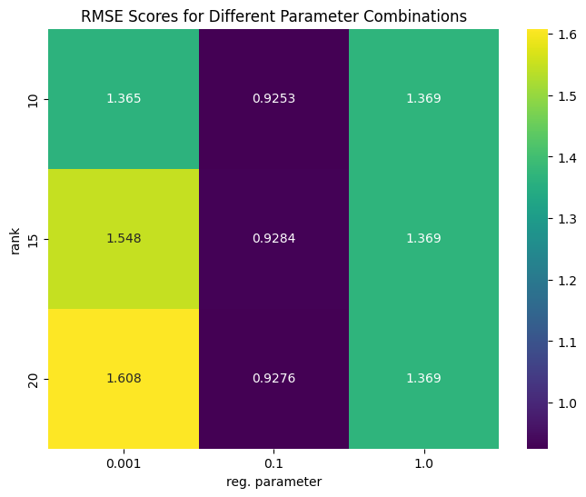
From this visualization, you'll typically see that RMSE first decreases and then increases as rank increases (due to overfitting). The optimal combination often balances model complexity with regularization.
Top-K Recommendations in Practice
Recommendations for All Users
# Generate top-10 recommendations for all users
recommendations_all = model.recommendForAllUsers(10)
recommendations_all.show(5)
Recommendations for Specific Users
# Get recommendations for a subset of users
selected_users = train.select(COL_USER).distinct().limit(3)
recommendations_subset = model.recommendForUserSubset(selected_users, 10)
recommendations_subset.show()
Performance Considerations
Moving recommendation systems to production introduces significant performance bottlenecks, primarily due to the massive scale of computation. Scoring all possible user-item pairs (a cross join) is often infeasible; for a million users and 100,000 items, this would mean 100 billion predictions.
Key challenges include:
- Computational Complexity: The sheer volume of user-item combinations makes exhaustive scoring incredibly time-consuming.
- Inefficient Calculations: Many systems compute recommendations sequentially instead of using optimized matrix multiplication libraries (like BLAS), failing to leverage hardware vectorization.
- Memory Usage: Large user and item factor matrices, along with intermediate calculations, can easily exhaust memory resources.
To mitigate these issues, production systems often employ strategies like using approximate algorithms (e.g., locality-sensitive hashing) to reduce computation, implementing matrix block multiplication for faster calculations, and pre-computing recommendations for active users during off-peak hours, serving cached results when possible.
Deploying ALS in Production Environments
Moving from a successful prototype to a production recommendation system involves several critical considerations that can make or break your deployment.
The Cold Start Challenge
One of the first issues you'll encounter in production is handling new users and items that weren't present during training. ALS provides built-in strategies through the coldStartStrategy parameter. You can choose to drop predictions for unknown users or items, which ensures clean evaluation metrics but might hurt user experience. Alternatively, you can allow NaN predictions and handle them in your application logic, perhaps falling back to popularity-based recommendations or content-based methods.
# Drop new users/items during prediction
als = ALS(coldStartStrategy="drop", ...)

# Or use NaN predictions for new users/items
als = ALS(coldStartStrategy="nan", ...)
Keeping Your Model Fresh
User preferences constantly change, so your model must adapt. While simple batch retraining (weekly or monthly) is a common approach, it can miss short-term trends. For more dynamic needs, consider incremental updates that incorporate new data without a full retrain. Hybrid systems, which combine collaborative filtering with content-based methods, can also provide more robust and fresh recommendations.
Monitoring What Matters
Effective monitoring goes beyond technical accuracy metrics like RMSE or Precision@K. While useful, these don't always reflect business value. Prioritize business-focused metrics such as click-through rates, conversion rates, and user engagement. Additionally, track recommendation diversity to avoid filter bubbles and catalog coverage to ensure you are promoting a wide range of items.
Conclusion
The Alternating Least Squares algorithm represents a perfect blend of mathematical elegance and practical utility. By decomposing the user-item interaction matrix into latent factors, ALS captures the hidden patterns that drive user preferences while remaining computationally tractable for large-scale deployments.
Key takeaways from our deep dive:
- Mathematical Foundation: ALS transforms a complex non-convex optimization into manageable convex subproblems
- Practical Implementation: PySpark's ALS provides a production-ready implementation with built-in distributed computing
- Parameter Tuning: Systematic grid search helps find optimal hyperparameters for your specific dataset
- Performance Considerations: Understanding computational bottlenecks is crucial for production deployment
Whether you're building the next Netflix or optimizing product recommendations for e-commerce, ALS provides a robust foundation for collaborative filtering that has stood the test of time in real-world applications.
The algorithm's success lies not just in its mathematical rigor, but in its ability to uncover the latent connections between users and items that drive human preference - turning the art of recommendation into a science.
Discussion